
Overview #
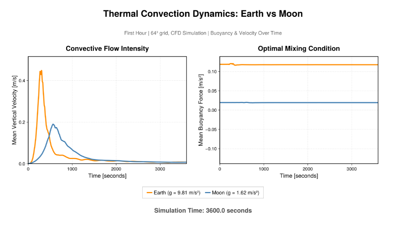
I built a GPU-accelerated simulation pipeline to study buoyancy-driven convection and volatile transport under lunar gravity, with Earth vs Moon comparisons using matched initial conditions.
Why? Because the core problem is Rayleigh-Benard convection 1, which is very well understood on Earth’s surface, understanding it for the Lunar surface is lacking. We have done this experiment in space on the ISS 2, that was not representative of true lunar gravity. Additionally there was some expectation that the Marangoni Effect which normally doesn’t affect the system on our gravity, would start dominating (this was actually confirmed by our simulations!)
This started as a personal simulation + visualization project: I wanted a clean, GPU-native RBC baseline under reduced gravity, then layered on a passive volatile tracer to see how transport and escape behavior change as the flow develops.
Aqualunar outcome #
This work supported LunaPure, the Aqualunar system developed by Canadian Strategic Missions Corporation (CSMC) with Pacific Rim Space Exploration Corp. (PARSEC). LunaPure won the Canadian Space Agency’s Aqualunar Challenge. The official challenge page lists Canadian Strategic Missions Corporation as the Stage 3 Grand Prize Winner for “LunaPure - A sustainable system to purify lunar water from the lunar polar regions.”
- Official Impact Canada Aqualunar Challenge page
- Canadian Space Agency Aqualunar Challenge page
- My LinkedIn post on the project
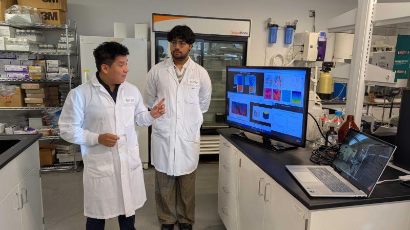
Presentation #
CFD notes #
This is straight-up computational fluid dynamics: solve the (incompressible) Boussinesq Navier-Stokes equations in a heated box, then postprocess + visualize.
- Governing physics: nonhydrostatic, incompressible flow with buoyancy from a temperature (or buoyancy) tracer; optional passive volatile tracer for transport/escape experiments.
- Numerics: structured grid + pressure-projection (Poisson solve) loop; stability managed by CFL-aware time stepping.
- Advection + time integration: WENO advection with Runge-Kutta stepping in Oceananigans for the production 3D runs.
- Turbulence modeling: subgrid closure for high-Rayleigh regimes; simpler scalar diffusivity closure when the flow stays tame.
- Compute + I/O: CUDA GPU runs, JLD2 field outputs, and Makie scripts for slice/volume diagnostics and Earth vs Moon comparisons.
Physics model #
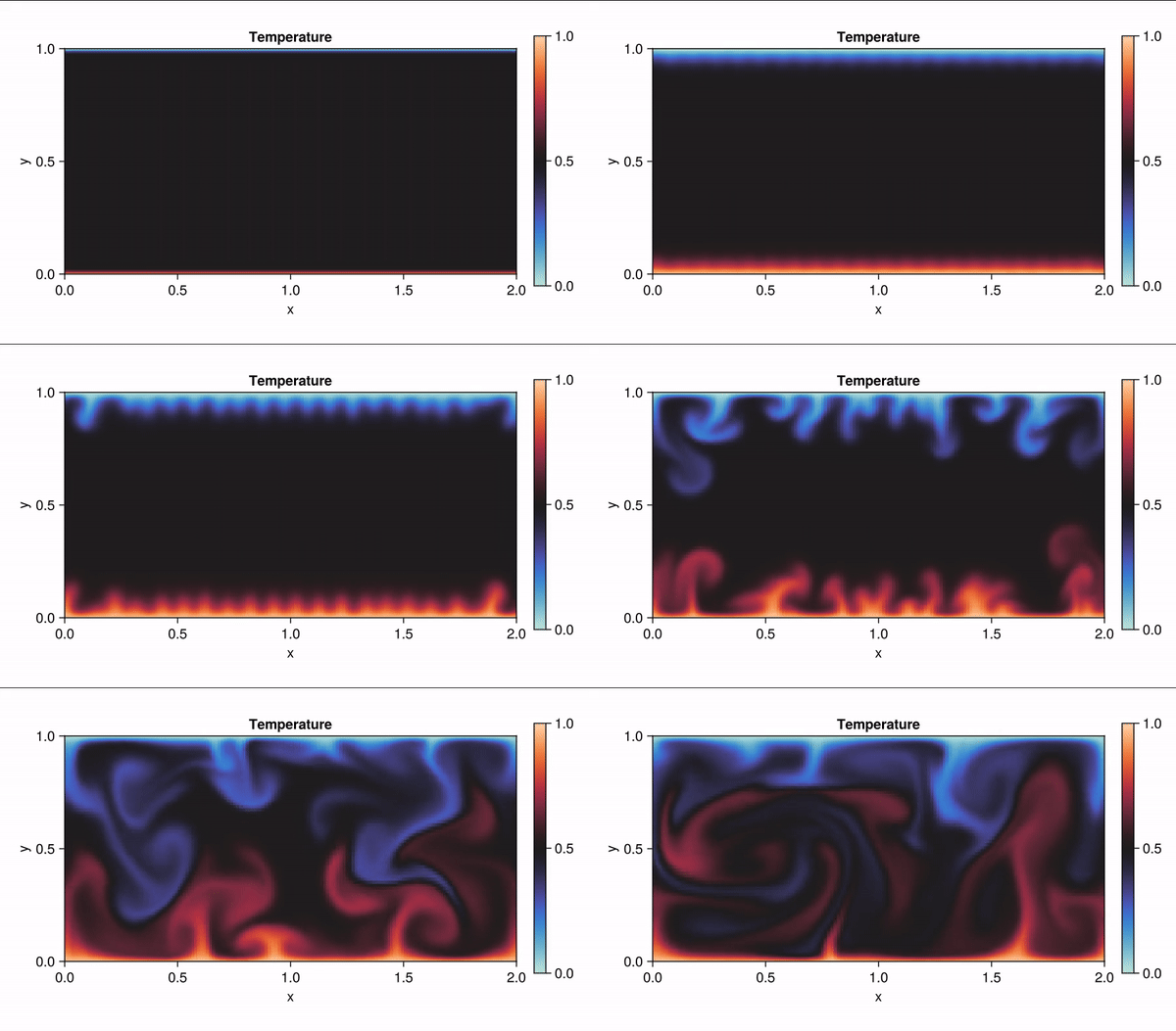
RBC in a closed box: hot bottom, cold top, periodic lateral boundaries, bounded vertical direction. I used the Boussinesq approximation so density variations only appear in the buoyancy term, with buoyancy defined from thermal expansion and gravity relative to a reference temperature. The initial condition is a linear stratification plus small random perturbations to trigger instability and roll-up.
For high Rayleigh regimes I used subgrid turbulence closures to model unresolved eddies. In lower regimes I used a simpler scalar diffusivity closure. I also added an optional vapor/volatile tracer that is advected by the flow, initialized with higher concentration near the hot boundary, and given a free-outflow (zero-gradient) condition at the top to model escape.
Why did I use a subgrid closure? Actually this was to fix a bug that wasn’t a bug. A previous simulation in 2D kept having bubbles pop up as the water boils but my system didn’t have that. It was a wild goose chase to find whether the eddies were disappearing because my resolution wasn’t tiny enough, but no, that wasn’t it- it was because their Rayleigh number was low due to their 2D nature, but oh well, it was a fun learning experience.
This was for single fluid physics, multi fluid is possible with multiple of these systems combined, but has never been attempted by any user of IncompressibleNavierStokes.jl or Oceananigans.jl as far as I am aware. Multi-fluidics was important to this project, but was accomplished via Ansys in a 2D sliced demo. The big upgrade of this versus Ansys however was the move from 2D to 3D, and the performance speed upgrade from using a commerical software (source: ran this in on my laptop RTX 4050) and the pure customization capability compared to Ansys.
Modeling evolution #
Phase 1: IncompressibleNavierStokes.jl (2D prototype) #
I started with a 2D Rayleigh-Benard prototype using IncompressibleNavierStokes.jl:
temperature_equationwith nondimensional parameters (Pr, Ra, Ge) and Dirichlet boundary conditions at the hot and cold plates.- Symmetric boundary conditions in the lateral direction and a
tanh_gridto cluster points near thermal boundary layers. - Live diagnostics: Nusselt number at both plates and a time-evolving mean temperature profile.
- Realtime plots and animation for fast iteration, with CPU and CUDA backends tested.
This stage was about verifying the physics and boundary conditions before moving to 3D.
Phase 2: IncompressibleNavierStokes.jl (3D attempt) #
I attempted the 3D extension with periodic boundaries in x/y and Dirichlet boundaries in z, plus a direct Poisson solver and RK3 time integration. The 3D path was promising but became brittle and effectively unmaintained for my use case, so I moved the full production model to Oceananigans.
Phase 3: Oceananigans.jl rework (production) #
Oceananigans gave me the GPU-native, nonhydrostatic 3D model I needed:
NonhydrostaticModelwith a buoyancy tracer and explicit boundary conditions.- WENO advection with Runge-Kutta time stepping.
- Subgrid closure (
AnisotropicMinimumDissipation) for high Rayleigh regimes; scalar diffusivity for simpler runs. - Adaptive time stepping with
TimeStepWizardfor CFL stability, plus fixed-timestep runs for consistent output cadence. - JLD2 time-series outputs of velocity and buoyancy fields for analysis and visualization.
Diagnostics + visualization #
- Compute Rayleigh number to classify regime and choose closures.
- Track maximum vertical velocity to monitor stability.
- Estimate vapor escape by integrating positive vertical flux at the top boundary (GPU fields copied to CPU for safe reduction).
- Makie-based visualization scripts for XY/XZ/YZ slices, consistent color scales, and side-by-side Earth/Moon comparisons.